After defining quarterback (QB) success in my previous article, it is now time to project QB play for the top prospects heading into the 2024 NFL draft. Last year, I developed a linear regression model to predict NFL success (defined as a 50-50 composite of EPA/play and average PFF grade). After optimizing with the greedy algorithm and manually eliminating collinearity issues, my model had an adjusted R^2 of 0.55. While this was a step in the right direction, there were several issues, mainly overfitting biases, that I will be correcting in this analysis.

Data Processing

To start, the dataset had a career minimum of 650 plays and 250 for each season. This restricted the sample size to only 29 QBs. Therefore, this dataset (same as for the previous article) uses 400 min. career plays and 150 min. for each season. This allows us to increase the sample size to 47 and include players who didn’t have as many plays due to them being bad. I also reduced the number of college single season plays from 200 to 150. (Keep in mind, the sample size is so small because college data is from 2014-2023. Hence, players like Cam Newton, Andrew Luck, or even Tom Brady won’t be studied here. This is perhaps the biggest issue that still hasn’t been solved.)

After these restrictions were set, I needed college stats that could be used as potential predictors. The PFF datasets I have access to provide information like big-time-throws, pressure-to-sack-rate, and grades. Not many tweaks were made to these individual stats, however one big change was considering different samples. Not only will I include the career play of these QBs, but I will also include first, last, worst, and best college season summaries. On top of this, the cfbfastR data I used last year only considers a handful of stats. This year, I’m expanding this list to include total EPA, sack plays, and even ground plays (sack or rush). I’m also considering career, first, last, worst, and best season splits.

One key predictor to NFL QB play is draft position. Draft pick has a -0.35 correlation with NFL success (defined as value per game metric, min. 10 games) since 1980. Thus, I will add in pick, round, and age from the nflfastR draft picks package.

Other potential predictors can include Combine measures, but they were not considered in this analysis. Tej Seth of SumerSports wrote about recent correlations with NFL success here.

Correlations

This dataset has 193 potential predictors that it is considering. So, let us look at those whose absolute correlation is 0.25 or larger.

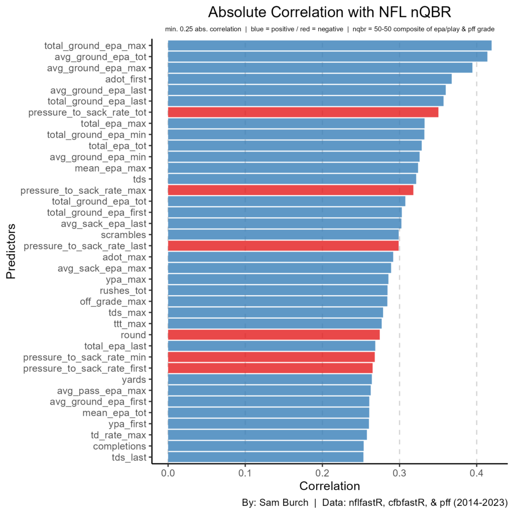
Right away, we can see that ground EPA is very important. Variants of ground EPA make up the top-3 and five of the top-6. In fact, the top-2 have a correlation above 0.40, which is great for football data. Pressure-to-sack-rate (PTSR) is seventh highest at -0.35, meaning the lower the better. This all points to pocket awareness — maximizing sack avoidance and scrambling — translates to the NFL. (Keep in mind, something like EPA per pressure play is more likely to determine how a QB plays under pressure; this is due to pressures that result in passes. However, I do not have access to pressure play-by-play data.) Average depth of target (ADOT) in their first year shows up surprisingly well at 0.37. This likely points to the importance of arm strength in the NFL. Total EPA and EPA per play have appearances high, which makes sense as these are based on overall production. Lastly, other total statistics — like TDs, completions, and yards — signal the importance of experience and productivity.

Draft round and pick were relatively low, at -0.27 and -0.25 respectively, when we know these should be high. If we look at the top correlations with pick, this may provide some traits our models may be missing on.

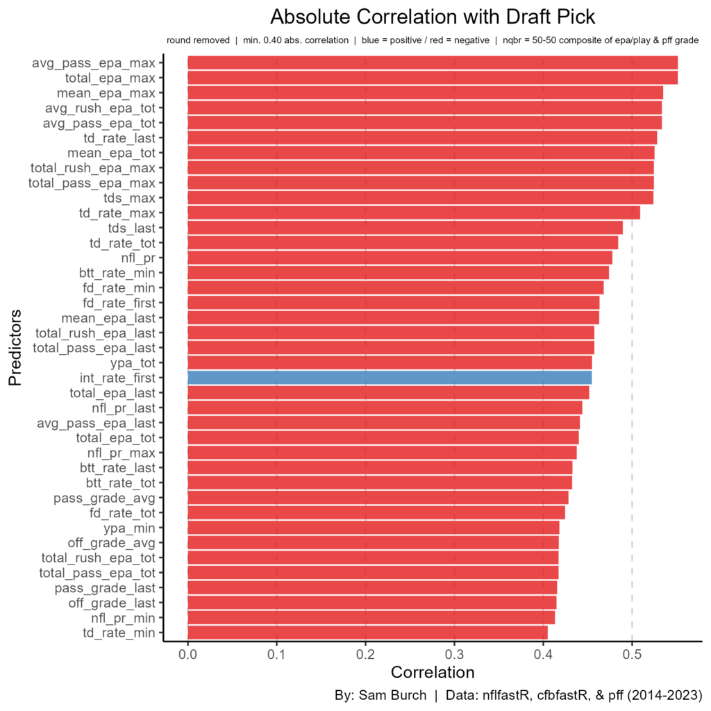
There are a lot of high correlations here, as nearly 40 other predictors have an absolute correlation above 0.40 with draft pick. The highest, above 0.50, include the following: average pass EPA in best year, total EPA in best year, EPA per play in best year, EPA per rush, and EPA per pass. Across the board, these statistics are production based whether that be through film (PFF grading) or analytics (EPA). This of course makes sense and likely will be more helpful statistics than just looking at sack avoidance. While that may ring true, it is possible NFL teams are underrating the importance of pocket awareness, experience, and maybe even arm strength as these have higher importance to NFL success in this dataset.

Data Mining

Let’s run through some interesting graphs before we begin modeling. For these, I will look at the 47 NFL QBs in the dataset along with the top-7 2024 draft prospects. In my last article, the 67th percentile was defined as the average starter, so we will continue to use this definition here.

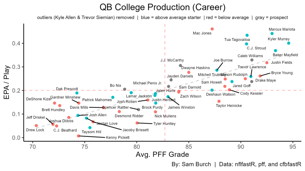
Looking at career production, Williams is atop, with Maye being second in grading and McCarthy being second in efficiency. While good production in college doesn’t necessarily translate to NFL production — look at the mix of blue and red dots in the top right and bottom left — we know that production is important for draft position. Thus, with draft position being important historically, we know college production should lead to better prospects in general.

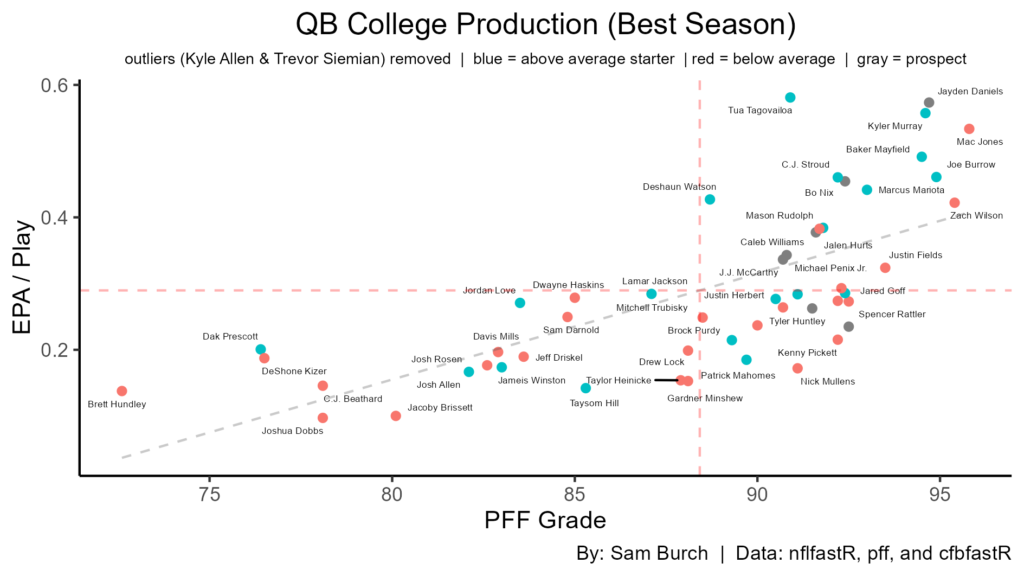
Looking at best season production for efficiency and grading, Daniels is by far the best of the 24′ prospects. Nix is second, followed by a cluster including Williams, Penix, and McCarthy. Maye & Rattler had elite grading in their best seasons, but efficiency was below average here. Regardless, all of these prospects have had good best seasons, which should be a good sign.

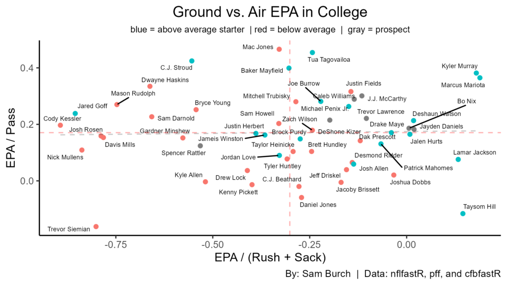
Here, we look at where on the field a QBs efficiency is coming from. The top right (good passing, rushing, and sack avoidance) is where one wants to be. Of the NFL QBs, only three are below average and six are above average. All of the 24′ prospects, except Rattler, are in this quadrant. Also, having good ground efficiency gives QBs a solid floor, since very few above average starters had below average ground efficiency and 8 of the top 9 were above average starters. Nix and Daniels show up the best in ground efficiency giving them a solid floor. Keep in mind though, some of the *successful* QBs with great ground EPA include Hill and Mariota.

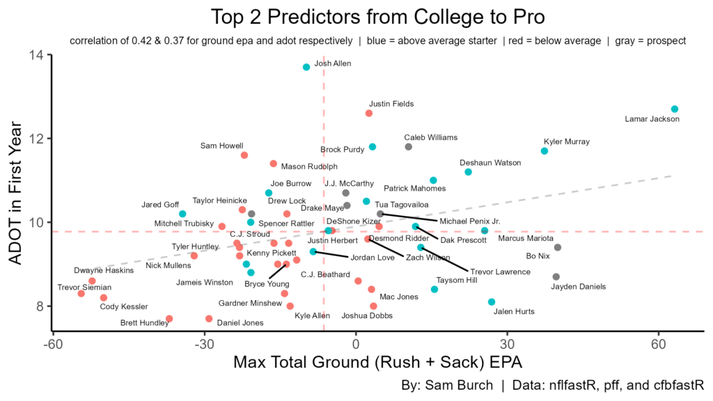
The top couple predictors are all dealing with ground efficiency. However, ADOT in a QBs first year is very high as well. As we compare the two, we can see there have only been three failures in the top right quadrant, compared to nine successes.  Williams, McCarthy, Maye, and Penix are all in this area. Nix and Daniels don’t have a high ADOT in their first year, however they have the second and third best max total ground EPA respectively. Again, this should lead to a high floor and is a good sign regardless of their ADOT.

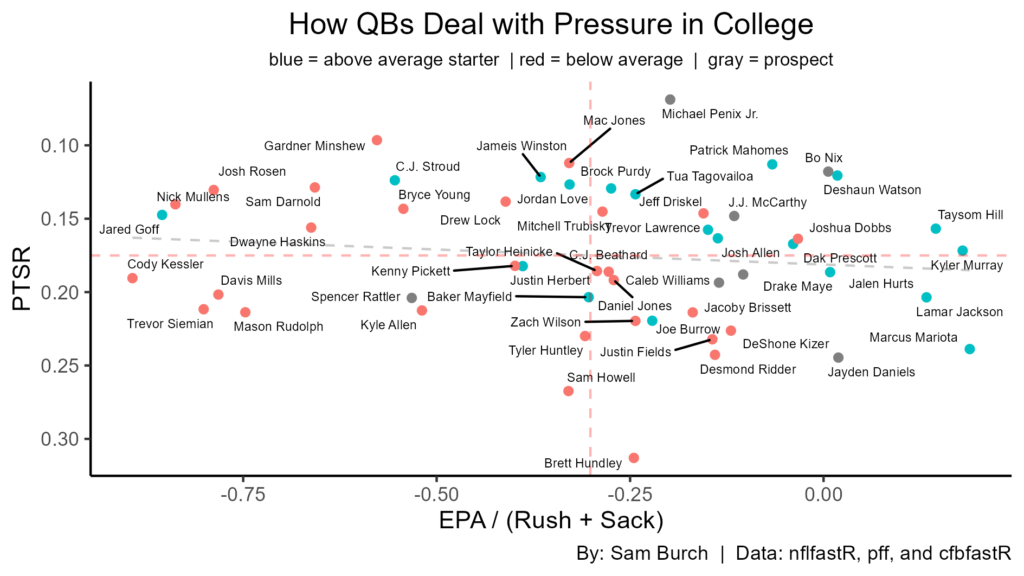
Just looking at how QBs deal with pressure in college can tell us a lot. Penix has the best PTSR in this entire dataset. Nix also doesn’t take many sacks and has the added benefit of his rushing. While Daniels has elite rushing too, he takes a lot of sacks. McCarthy has good (not great) sack avoidance, while Williams and Maye are on the border between good and bad. Rattler’s below average in both, which is concerning.

Before moving onto modeling, let’s see how draft position tends to NFL success. 15 of the 25 QBs drafted in round 1 become above average NFL starters. Meanwhile, only 4 of the 22 non-first rounders become above average starters. Hurts and Prescott were genuinely non-first round hits. Purdy still has something to prove after only playing with an elite offense around him. Hill is just efficient on a small sample. These players skew the correlations in recent history, along with first-round busts. However, they will be kept in the sample as we move onto modeling because of the already small sample of QBs in the dataset. Regardless, if NFL teams don’t value a QB as a first rounder, this is a bad sign. This will be important when it comes to players like Nix and Penix, as they are fringe first rounders.

Modeling

For our train-test split — not considered last year due to a small sample size — we will use 85-15. The training set needs to have enough data points, otherwise the results will not be trustworthy. However, our testing results cannot be fully trusted here. While they can provide some small signal, it will likely be very noisy due to a small sample. Thus, we must keep this in mind when doing model selection.

To get an idea of what a good RMSE and r^2 might look like, when we use the average (0.547) to predict QB success. We get an RMSE of 0.348. This means, on average, we are off by ~35 on a scale from 0-100 (aka percentile).

Linear Regression

For the linear regression we can’t fit a model with all the potential predictors, because of dimensional issues. Therefore, we start by fitting one with predictors where their absolute correlations are 0.275 or more. Then, by optimizing using the greedy algorithm this gives us the following: an adjusted r^2 of 0.466 and a RMSE of 0.232. The adjusted r^2 is very good and the error is not bad, but collinearity is a problem. Hence, it is not smart to consider this model in the model selection later now.

This model considers predictors with an absolute correlation above 0.30. When optimizing, again with the greedy algorithm, the adjusted r^2 is 0.343 and the error is 0.260. Their numbers are both good. The diagnostics pass here, so this is an improvement over the last model. The predictors selected here are average ground EPA, total EPA, and PTSR.

Using the maximum total ground EPA as the only predictor, we get an RMSE of 0.34. The adjusted r^2 is 0.19, which isn’t awful. If we instead use PTSR as the only predictor, the r^2 drops to 0.05, but the error improves to 0.31. When using draft pick, both r^2 and RMSE are bad — 0.01 and 0.33 respectively. Considering these factors, I will try to construct a model which has a high adjusted r^2, low RMSE, and low collinearity error. This will not be perfect, and is not recommended as it will introduce bias, although it will be an interesting exercise.

Again, this process is not ideal, but I looked at the top correlations and did trial and error to optimize r^2 and the prediction error. I ended up with PTSR, average ground EPA, ADOT in first year, and total EPA in best year as the predictors. (Total EPA in best year had a high correlation with round and a better trade off with the comparison metrics.) This model has an adjusted r^2 of 0.321, RMSE of 0.240, and low collinearity. If I run the greedy algorithm on this model, it suggests to drop total EPA in best year. This would improve the r^2 to 0.326, but the RMSE would worsen to 0.251. Thus, we will keep this predictor considering the better RMSE and the tell of overall play, on top of pocket awareness and arm strength. 

Lasso

We will next consider a lasso regression, as not all of these predictors should be included due to their massive collinearity.

After completing Lasso, this tells us that no predictors are worth keeping. The intercept (0.53) is what the model will predict each time. By doing so, the error is 0.353; this is worse than our average model.

KNN

The prediction error for KNN was optimized at K = 22. This led to an error of 0.343, again not great.

Random Forest

After tuning on mtry and nodesize, the selected model has an r^2 of 0.031, with an OOB rate of 0.082. The rmse is bad too at 0.386. So, while this model won’t be selected, the top variables for this model include EPA totals, ADOT, and completion percentage (CP).

XGBoost

The best prediction error for XGBoost also does not perform with an error of 0.366. The optimal tuning here was 0.1 ETA, 5 max depth, and 2 ntrees.

Model Selection

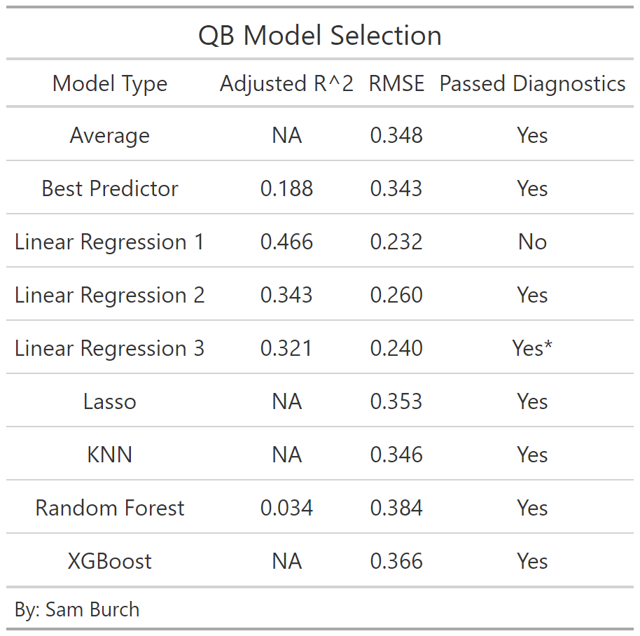
Across the board, most models perform very similarly. Looking at adjusted r^2, the first linear regression (which included all predictors with an abs. correlation of 0.275 or higher) is by far the best at 0.466. However, there are certainly overfitting issues as the model does not pass the collinearity diagnostics. Next tier here is the second and third linear regression respectively. These have good r^2s, but not great at around a third. 

For prediction error, the baseline is 0.348 for the average. Five models did perform better than this. The best here was the first linear regression, however note the collinearity issues. Next comes the other linear regression models, with this time the third performing slightly better. With the testing sample size being so small, this RMSE statistic should be taken with a grain of salt though.

Therefore, we will select the second linear regression model, with hesitancy. This model has the second highest adjusted r^2 and the third lowest prediction error. The first LR model would have been chosen, but it did not pass the collinearity diagnostics. Meanwhile, the third linear regression model does have a better RMSE, however the more stable stat (r^2) is worse than the second LR. On top of this, bias was introduced when modeling the third linear regression. The runners up are the average, the best predictor, and the KNN model. The best predictor and KNN model each had a slightly better prediction error than the average. Although that is the case, the errors are all close enough that the average is probably the best of the runner ups. The advanced models all didn’t perform well. This can possibly be improved by transforming the predictors into principal components. However, it is not necessary as the advanced models all pass the diagnostics by tuning them.

Projections

Let’s see how the selected model projects the 2024 NFL draft prospects!

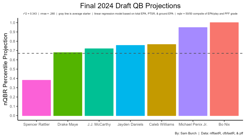
Nix and Penix are in their own tier due to their elite pocket awareness and experience. The issue with both is their consensus rankings have them as fringe first rounders. Considering this, if they fall out of the first round, they shouldn’t necessarily be looked at as values. The top-4 on the consensus board are next at slightly above average. McCarthy is hurt by his limited number of plays, same with Williams and Maye, but Daniels is helped by it. Tak on the fact that all have had elite seasons makes them good prospects. The biggest issue is Daniels needs a good surrounding as his PTSR is concerning low. Daniels’ experience and rushing should help him though. Williams and Maye weren’t elite in pocket awareness in college, but their elite production makes them elite prospects regardless. McCarthy was great across the board, but it was on a small sample, as stated earlier. On the other hand, Rattler projects poorly in every category but PTSR.

Some late round QBs are interesting. Jordan Travis has the third highest projection (77th percentile) out of the 11 prospects considered, due to his experience and good (not great) pocket awareness. The other three (Hartman, Pratt, and Milton) all project as below average starter or backup. Hartman and Pratt are helped by their production & experience, but hurt by their pocket awareness, which is concerning. Milton might be worth a flyer with his strong arm and decent pocket awareness.

Conclusion

Next steps include using a larger sample, implementing principal components into the models, and adding even more predictors. The first is by far the most important, as having a larger sample size will almost certainly create a better model than using the average. Implementing PCs will help the advanced models perform better. More predictors, like performance in a clean pocket, on play action plays, or percentage of pressures assigned to the QB will likely have some significance. Regardless, this analysis is a big step forward from last year’s and provides us with a more concrete projection of the QB prospects. One continued theme is the stability of pocket awareness. Metrics like PTSR and ground EPA need to be considered more when ranking prospects. 

Thanks for reading!

By: Sam Burch

Twitter (@sburch323)

GitHub (@burchsam)